| 1761 |
Global |
Marine chronometer |
Geographical Features: Landmarks and Ecosystems
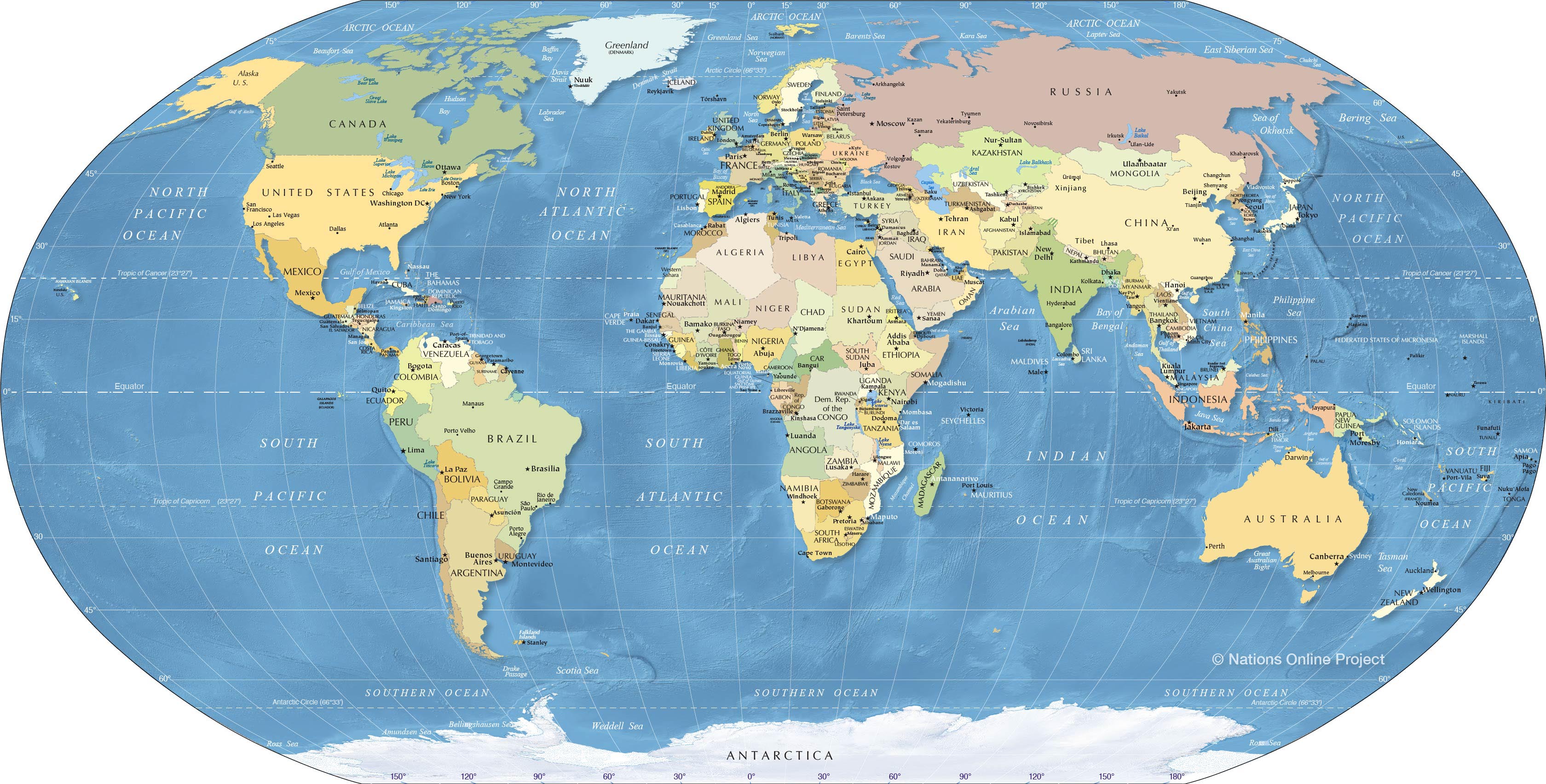
Geographical features define the physical identity of continents, shaping biodiversity, climate systems, and human civilizations. Natural landmarks such as mountain ranges, river basins, and deserts serve as ecological hotspots and geopolitical boundaries, while unique ecosystems—ranging from tropical rainforests to polar tundras—host extraordinary biological diversity. This section categorizes significant geographical features by continent, examines their ecological roles, and presents a structured framework for comparative analysis. Extreme geographical points—such as the highest peaks or deepest trenches—highlight the stark contrasts in continental topography, underscoring their influence on global environmental dynamics.
Significant Natural Landmarks by Continent
Natural landmarks act as focal points for geological, hydrological, and ecological processes. Below is a categorized overview of the most prominent features across continents, emphasizing their geographical and cultural importance.Africa
Mount Kilimanjaro (Tanzania) – Highest free-standing mountain in the world (5,895 m), a dormant volcano with glaciers that reflect climate change impacts.
Amazon Basin (South America) – Largest tropical rainforest, spanning nine countries, with the Amazon River (6,400 km) as its lifeline.
Great Rift Valley (East Africa) – A tectonic depression hosting Lake Victoria, the Nile’s headwaters, and fossil-rich sites like Olduvai Gorge.
Atacama Desert (South America) – Driest non-polar desert, with hyperarid zones and unique halophilic flora adapted to extreme aridity.Asia
Himalayas (South Asia) – Home to Mount Everest (8,848 m), the world’s highest peak, acting as a climatic barrier influencing monsoons.
Siberian Taiga (Russia) – Largest boreal forest, storing 30% of global terrestrial carbon and sustaining diverse fauna like brown bears and Siberian tigers.
Dead Sea (Middle East) – Lowest land point on Earth (−430 m), a hypersaline lake with therapeutic mineral deposits.
Ganges-Brahmaputra Delta (South Asia) – World’s largest delta, critical for agriculture and biodiversity, facing threats from sediment deposition and sea-level rise.Europe
Alps (Central Europe) – Youngest major mountain range, shaping drainage systems for the Rhine, Danube, and Po rivers, with glacial carving defining its peaks.
Scandinavian Peninsula (Nordic Countries) – Northernmost landmass in Europe, featuring fjords like Norway’s Geirangerfjord and vast boreal forests.
Iceland’s Volcanic Landscape – Home to active volcanoes (e.g., Eyjafjallajökull) and geothermal areas, including the Geysir geothermal field.
Black Sea Coastal Wetlands (Ukraine/Romania) – Ramsar-listed sites like the Danube Delta, supporting migratory birds and endangered species like the European mink.North America
Rocky Mountains (USA/Canada) – Continental divide influencing river flow (Mississippi vs. Pacific drainage) and hosting alpine ecosystems.
Grand Canyon (USA) – Carved by the Colorado River over 6 million years, exposing 2 billion years of geological history.
Yucatán Peninsula (Mexico) – Features cenotes (sinkholes) linked to the Chicxulub impact crater and Mayan archaeological sites.
Great Lakes (USA/Canada) – Largest freshwater system by surface area, containing 21% of the world’s surface freshwater.South America
Andes Mountain Range – Longest continental range (7,000 km), with Aconcagua (6,961 m) as the highest peak outside Asia.
Pantanal Wetlands (Brazil/Bolivia) – World’s largest tropical wetland, with seasonal flooding supporting jaguars and hyacinth macaws.
Atacama Desert (Chile) – Contains the driest place on Earth (Yungay) and the world’s largest astronomical observatory (ALMA).
Amazon Rainforest (Brazil/Peru/Colombia) – Produces 20% of global oxygen, with over 400 billion trees across 5.5 million km².Australia & Oceania
Great Barrier Reef (Australia) – Largest coral reef system, spanning 2,300 km and supporting 1,500 fish species and 400 coral types.
Uluru-Kata Tjuta (Australia) – Sacred sandstone monoliths in the Red Centre, with geological formations dating back 600 million years.
Tasman Glacier (New Zealand) – Longest glacier in New Zealand, retreating due to climate change and feeding into Lake Pukaki.
Kermadec Islands (New Zealand) – Remote volcanic islands with unique seabird colonies and deep-sea hydrothermal vents.Antarctica
South Pole (Amundsen-Scott Station) – Geographic South Pole (−2,835 m elevation), with the coldest recorded temperature (−89.2°C at Vostok Station).
Transantarctic Mountains – Natural divide separating East and West Antarctica, with the Beardmore Glacier as a key route to the pole.
McMurdo Dry Valleys – Polar deserts with almost no ice or snow, hosting extremophile microbes and serving as a Mars analog study site.
Unique Ecosystems: Climate, Biodiversity, and Human Impact
Ecosystems are defined by their climate regimes, species adaptations, and anthropogenic pressures. Below are case studies of globally significant ecosystems, structured by their defining characteristics and conservation challenges.Tropical Rainforests
Amazon Rainforest (South America)
Climate: Equatorial (20–30°C year-round, 2,000–3,000 mm annual rainfall).
Biodiversity: 10% of known species, including jaguars, harpy eagles, and 16,000 tree species.
Human Impact: Deforestation (17% lost since 1970), driven by agriculture (soy, cattle) and mining. Threat: Loss of carbon sequestration and indigenous displacement.
Ecological Significance: Regulates global climate, produces medicines (e.g., quinine), and hosts uncontacted tribes.- Congo Rainforest (Central Africa)
Climate: Humid tropical (25–30°C, 1,500–2,000 mm rainfall).
Biodiversity: Home to gorillas, bonobos, and 600 bird species; high endemism in flora (e.g., Gnetum species).
Human Impact: Logging (rosewood, okoumé) and artisanal mining. Threat: Ebola outbreaks disrupting conservation efforts.
Ecological Significance: Second-largest carbon sink after the Amazon; critical for Congo River hydrology.Deserts
Atacama Desert (South America)
Climate: Hyperarid (<0.1 mm annual rainfall), with temperature extremes (−20°C to 40°C).
Biodiversity: Halophytes (e.g., Tillandsia) and nocturnal fauna (e.g., vicuña). Endemic species like the Atacama toad.
Human Impact: Lithium mining (for EVs) and tourism. Threat: Over-extraction of groundwater and light pollution affecting astronomy.
Ecological Significance: Natural laboratory for astrobiology; unique microbial extremophiles.- Sahara Desert (Africa)
Climate: Arid to hyperarid (10–50 mm rainfall), with sand dunes (e.g., Erg Chebbi) and regs (stone plains).
Biodiversity: Fennec foxes, dorcas gazelles, and Saharan cheetahs. Ephemeral oases support date palms and acacia trees.
Human Impact: Nomadic pastoralism and fossil fuel extraction. Threat: Desertification expanding southward by 50 km/year.
Ecological Significance: Acts as a climatic barrier; historical trade routes (e.g., Trans-Saharan) shaped civilizations.Polar and Alpine Ecosystems
Arctic Tundra (North America/Eurasia)
Climate: Cold (0°C to −40°C), with permafrost and short growing seasons (3–5 months).
Biodiversity: Caribou, Arctic foxes, and migratory birds (e.g., barnacle geese). Lichen and moss dominate vegetation.
Human Impact: Oil drilling (e.g., Prudhoe Bay) and melting sea ice. Threat: 3°C warming since 1970; habitat loss for polar bears.
Ecological Significance: Carbon sink (permafrost stores 1.5 trillion tons of carbon); indicator of climate change.- Himalayan Alpine Meadows (Asia
Cultural and Political Divisions
The interplay between cultural heritage and political boundaries has profoundly shaped continental geography, often reflecting historical power struggles, indigenous sovereignty, and colonial legacies. Political subdivisions—such as nation-states, territories, and autonomous regions—emerge from complex negotiations between governance, ethnicity, and territorial claims. Meanwhile, indigenous cultural regions, rooted in pre-colonial traditions, frequently overlap or conflict with modern borders, revealing the enduring tensions between tradition and statecraft. Colonial mapping practices further exacerbated these divisions by imposing arbitrary boundaries that disregarded existing cultural and ecological landscapes, leaving behind contested regions where sovereignty remains unresolved.
Political Subdivisions of Continents
The following table categorizes continents by their sovereign states, territories, and dependent regions, including key administrative details. Population figures are approximate (2023 estimates) and sourced from the United Nations, World Bank, and national censuses. Official languages listed reflect those recognized by governments, though regional linguistic diversity often exceeds these classifications.
| Continent |
Country/Territory |
Capital |
Population (approx.) |
Official Language(s) |
|---|
| Africa |
Algeria |
Algiers |
45.6 million |
Arabic, Berber (Tamazight) |
| Egypt |
Cairo |
112.7 million |
Arabic |
| South Africa |
Pretoria (executive), Cape Town (legislative), Bloemfontein (judicial) |
60.4 million |
English, Afrikaans, Zulu, Xhosa, etc. (11 official) |
| Nigeria |
Abuja |
227.9 million |
English |
| Ethiopia |
Addis Ababa |
126.6 million |
Amharic |
| Madagascar |
Antananarivo |
29.9 million |
Malagasy, French |
| Western Sahara |
Laayoune (disputed) |
600,000 (estimated) |
Arabic, Hassaniya Arabic |
| Asia |
China |
Beijing |
1.41 billion |
Standard Mandarin |
| India |
New Delhi |
1.43 billion |
Hindi, English |
| Indonesia |
Jakarta |
277.5 million |
Indonesian |
| Japan |
Tokyo |
123.3 million |
Japanese |
| Kazakhstan |
Nur-Sultan |
19.6 million |
Kazakh, Russian |
| Israel |
Jerusalem (disputed) |
9.3 million |
Hebrew, Arabic |
| Kashmir (Jammu and Kashmir) |
Srinagar (summer), Jammu (winter) |
13.3 million (India-administered) |
Kashmiri, Urdu, Hindi, Dogri |
| Europe |
Russia |
Moscow |
146.4 million |
Russian |
| Germany |
Berlin |
83.2 million |
German |
| France |
Paris |
68.4 million |
French |
| United Kingdom |
London |
67.7 million |
English, Welsh, Scots Gaelic, Irish |
| Iceland |
Reykjavik |
386,000 |
Icelandic |
| North America |
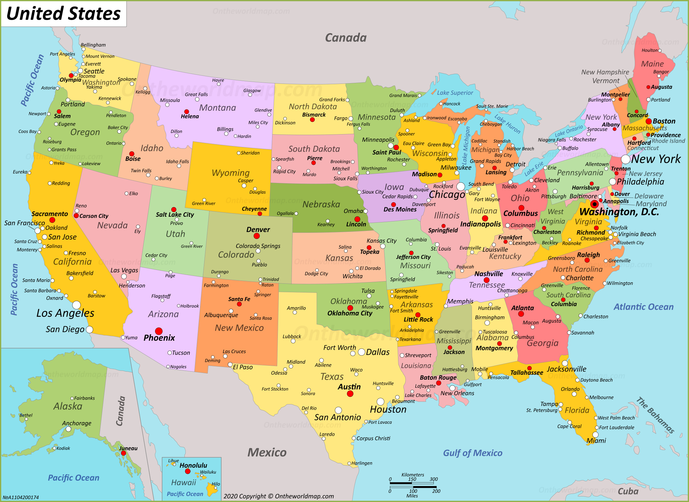
United States |
Washington, D.C. |
339.9 million |
English |
| Canada |
Ottawa |
38.8 million |
English, French |
| Mexico |
Mexico City |
128.5 million |
Spanish |
| Greenland |
Nuuk |
56,000 |
Greenlandic, Danish |
| Puerto Rico |
San Juan |
3.2 million |
Spanish, English |
| South America |
Brazil |
Brasília |
216.4 million |
Portuguese |
| Argentina |
Buenos Aires |
45.8 million |
Spanish |
| Peru |
Lima |
34.3 million |
Spanish, Quechua, Aymara |
| Oceania |
Australia |
Canberra |
26.4 million |
English |
| New Zealand |
Wellington |
5.1 million |
English, Māori, NZ Sign Language |
| Papua New Guinea |
Port Moresby |
10.3 million |
English, Tok Pisin, Hiri Motu |
| French Polynesia |
Papeete |
281,000 |
French, Tahitian |
Technological Advancements in Continental Mapping
The evolution of continental mapping reflects humanity’s pursuit of precision, scalability, and real-time data integration. From rudimentary celestial observations to satellite-enabled global surveillance, each technological leap has redefined cartographic capabilities. Modern advancements—such as GPS, drones, and LiDAR—now enable sub-meter accuracy, dynamic data fusion, and automated terrain analysis. This progression underscores the shift from static analog representations to dynamic, multi-spectral digital models, transforming mapping from a craft into a data-driven science. The integration of Geographic Information Systems (GIS) further democratized large-scale cartography, allowing governments, researchers, and industries to generate continental-scale topographic maps with unprecedented efficiency. Meanwhile, satellite constellations like Landsat and Sentinel provide continuous, high-resolution imagery, enabling applications from deforestation monitoring to urban expansion tracking. Below, the technical specifications of key tools, GIS workflows, and comparative analyses of analog vs. digital methods are examined, alongside the operational mechanics of satellite-based continental data acquisition.
Mapping tools have evolved in tandem with advancements in astronomy, physics, and computing, each era introducing instruments with distinct capabilities and limitations. Early cartography relied on celestial navigation devices, while modern techniques leverage electromagnetic sensing and computational algorithms. The progression can be categorized into five phases: pre-mechanical, mechanical, electro-optical, digital-sensor, and AI-augmented, each marked by breakthroughs in accuracy, coverage, and automation.
Key Metric for Comparison:
Accuracy (horizontal/vertical), Coverage Rate (km²/hour), Operational Range (local/continental/global), Data Output Format (analog/digital), and Cost per Unit Area (USD/km²).
-
Pre-Mechanical Era (Ancient–18th Century): Celestial and Triangulation Tools
Astrolabes, quadrants, and theodolites measured angles to celestial bodies or terrestrial landmarks, enabling early navigators to plot latitudes and longitudes. The marine chronometer (1761), developed by John Harrison, introduced time-based longitude calculation, reducing positional errors from hours to minutes.
Technical Specifications:
- Astrolabe: ±0.5° accuracy (equivalent to ~55 km error at equator).
- Theodolite (18th c.): ±1 arc-minute (~30 m error at 1 km distance).
- Limitations: Manual calculations, susceptibility to human error, and reliance on clear skies.
-
Mechanical Era (19th–Early 20th Century): Planimeters and Aerial Photography
The planimeter (1814) automated area calculations from hand-drawn maps, while aerial photography (1858, Nadar’s balloon flights) introduced large-scale terrain imaging. Stereoscopic plotting instruments (e.g., Wild A8, 1940s) combined overlapping photos to generate 3D models, achieving ±1 m accuracy in controlled conditions.
Technical Specifications:
- Aerial Photography (1930s): 1:50,000 scale, ±5 m RMSE (Root Mean Square Error).
- Limitations: Weather dependency, labor-intensive stereoscopic compilation, and lack of real-time updates.
-
Electro-Optical Era (Mid-20th Century): Radar and Early Satellite Imagery
World War II spurred advancements in radar altimetry (e.g., Shoran, 1940s) and side-looking airborne radar (SLAR, 1950s), enabling cloud-penetrating terrain mapping. The first civilian satellite (Landsat 1, 1972) provided multispectral imagery at 80 m resolution, revolutionizing continental monitoring.
Technical Specifications:
- Landsat MSS (1972): 80 m spatial resolution, 4 spectral bands (0.5–1.1 µm), revisit cycle: 18 days.
- Limitations: Low resolution, limited spectral range, and data processing delays.
-
Digital-Sensor Era (1980s–Present): GPS, LiDAR, and Hyperspectral Imaging
The Global Positioning System (GPS, 1995) introduced centimeter-level positioning, while LiDAR (Light Detection and Ranging, 1960s commercialized in 1990s) achieved sub-meter terrain modeling. Hyperspectral sensors (e.g., Hyperion, 2000) expanded spectral analysis to 220+ bands, enabling material classification.
Technical Specifications:
- GPS (Modern): ±1–5 mm horizontal/vertical (RTK correction), 24/7 availability.
- Aerial LiDAR (2010s): ±15 cm RMSE, 10–20 pts/m² density, 500 km²/day coverage.
- Satellite LiDAR (ICESat-2, 2018): 15 m footprint, 0.7 m vertical accuracy, global coverage.
-
AI-Augmented Era (2010s–Present): Machine Learning and Autonomous Systems
Deep learning models (e.g., U-Net for segmentation, Transformers for change detection) process satellite imagery at continental scales. Autonomous drones (e.g., DJI Matrice 300 RTK) integrate LiDAR, multispectral, and thermal sensors, while quantum sensors (e.g., atomic clocks for gravity mapping) push gravitational terrain modeling to ±1 cm accuracy.
Technical Specifications:
- Sentinel-2 (2015): 10–60 m resolution, 13 spectral bands, 5-day revisit.
- LiDAR Drones (2020s): ±5 cm RMSE, 100 ha/hour, AI-assisted point cloud classification.
Step-by-Step Procedure for Generating Continental-Scale Topographic Maps Using GIS
Generating a continental-scale topographic map via GIS involves data acquisition, preprocessing, spatial analysis, and visualization, leveraging tools like QGIS, ArcGIS Pro, or GRASS GIS. The workflow integrates satellite imagery, LiDAR, and DEM (Digital Elevation Model) datasets to produce seamless, multi-resolution terrain models. Below is a structured procedure with technical specifications for each stage.
-
Data Acquisition and Integration
Gather primary and secondary datasets from global repositories (e.g., USGS EarthExplorer, Copernicus Open Access Hub, ALOS World 3D). Key inputs include:
- Satellite Imagery: Sentinel-2 (10 m multispectral), Landsat 8/9 (30 m), or ASTER (15 m).
- LiDAR Data: ALOS PALSAR (5 m DEM), NASA’s SRTM (30 m), or airborne LiDAR (sub-meter).
- Auxiliary Data: HydroSHEDS (hydrology), OpenStreetMap (anthropogenic features).
Data Requirements:
- Spatial Coverage: Entire continent (e.g., Africa: ~30.37 million km²).
- Temporal Alignment: Multi-year composites to account for seasonal variations.
- Coordinate System: WGS84 (EPSG:4326) for global consistency; UTM zones for regional precision.
-
Preprocessing: Geometric and Radiometric Correction
Apply corrections to mitigate distortions and enhance interpretability:
- Orthorectification: Remove terrain-induced displacement using a DEM (e.g., SRTM 1Arc-Second) via ENVI or SNAP toolboxes.
- Atmospheric Correction: Apply FLAASH (Fast Line-of-sight Atmospheric Analysis of Spectral Hypercubes) for Landsat or Sen2Cor for Sentinel-2.
- Mosaicking: Stitch adjacent tiles using seamline algorithms (e.g., GCPs + RPC models in ArcGIS).
Technical Specifications:
- Orthorectification Accuracy: ±0.5 pixel (e.g., ±5 m for Sentinel-2).
- Radiometric Resolution: 12-bit (Landsat) or 16-bit (Sentinel-2) dynamic range.
-
DEM Generation and Terrain Analysis
Generate a high-resolution DEM using SRTM + LiDAR fusion or photogrammetry (e.g., Pix4Dmapper):
1. LiDAR Processing: Classify point clouds (ground vs. non-ground) using TIN (Triangulated
Practical Applications of Continental Maps
Continental maps serve as indispensable tools across disciplines, bridging theoretical geography with real-world utility. From facilitating cross-continental travel and scientific research to enabling disaster preparedness and resource management, their applications are diverse and impactful. This section explores how continental maps are leveraged in travel planning, logistical infrastructure, climate science, and survival strategies, with a focus on actionable frameworks and case studies.
Designing Travel Itineraries Using Continental Guides
Continental maps provide a macro-level perspective essential for crafting efficient and enriching travel itineraries, particularly for large-scale or multi-destination journeys. Seasonal variations in weather, wildlife activity, and cultural events dictate optimal timing for exploration. Below are structured recommendations for must-visit regions, categorized by season and continent, alongside logistical considerations for seamless travel execution.Seasonal Highlights and Logistical Considerations
Continental maps highlight temporal and spatial dynamics that influence travel planning. For instance, the Great Migration in the Serengeti (East Africa) peaks between July and October, aligning with dry seasons that concentrate herbivores around water sources. Conversely, Patagonia’s hiking trails (South America) are most accessible from November to March, when snowmelt reveals paths and temperatures are moderate. Below is a seasonal breakdown of key destinations, derived from climatological data and tourism trends:
"Timing is critical in travel planning: a map’s seasonal annotations can mean the difference between witnessing a once-in-a-lifetime natural phenomenon and encountering closed roads or extreme weather."
-
Africa: Wildlife and Cultural Pilgrimages
- Dry Season (June–October): Serengeti (Tanzania/Kenya), Okavango Delta (Botswana), Maasai Mara (Kenya). Focus on safari logistics, including game reserve permits and guided tours.
- Wet Season (November–May): Victoria Falls (Zambia/Zimbabwe), Gorilla trekking in Rwanda/Uganda. Prioritize water-based activities and health precautions (e.g., malaria prophylaxis).
-
South America: Adventure and Heritage
- Summer (December–February): Patagonia (Chile/Argentina), Amazon Rainforest (Brazil/Peru). Plan for high-altitude acclimatization and jungle navigation tools.
- Winter (June–August): Andes Mountain treks (Peru/Bolivia), Machu Picchu. Account for reduced daylight and potential road closures due to snow.
-
Europe: Historical and Scenic Routes
- Spring (April–June): Alpine hiking (Swiss/Austrian Alps), lavender fields (Provence, France). Book accommodations early for peak tourist seasons.
- Autumn (September–November): Northern Lights (Scandinavia), wine regions (Bordeaux, Tuscany). Leverage daylight savings for extended sightseeing hours.
-
Asia: Monsoon-Driven Travel
- Monsoon Season (June–September): Backwaters of Kerala (India), rice terraces of Bali (Indonesia). Plan indoor cultural experiences (e.g., temples, museums).
- Dry Season (November–February): Himalayan treks (Nepal/Bhutan), desert safaris (Rajasthan, India). Secure high-altitude permits and oxygen supplies if needed.
Itinerary Design Framework
A well-structured itinerary integrates:
1. Route Mapping: Use continental maps to plot connections between destinations, prioritizing efficiency (e.g., combining Nairobi and Serengeti in one trip).
2. Time Zones and Flight Paths: Align layovers with local time to minimize jet lag (e.g., eastbound travel from Europe to Asia should include gradual time adjustments).
3. Local Expertise: Consult regional guides or digital platforms (e.g., Lonely Planet, Wikivoyage) for real-time updates on road conditions, visa requirements, and cultural etiquette.
Logistical Resources for Continental Travel
Efficient travel relies on robust infrastructure, and continental maps provide a spatial context for identifying critical hubs—airports, ports, and road networks—that underpin connectivity. Below is a structured table of major logistical resources, categorized by continent, with capacity data and operational notes derived from official sources (e.g., ICAO, IATA, World Bank).
"Infrastructure capacity is a limiting factor in travel planning: a map’s annotated resources (e.g., runway lengths, port drafts) can preempt delays or logistical failures."
| Continent |
Resource |
Location |
Capacity |
Key Notes |
|---|
| Africa |
Airport |
Jomo Kenyatta International (Nairobi, Kenya) |
20 million passengers/year; 4 runways (1 x 4,500m) |
Primary hub for East African flights; limited night operations due to wildlife corridors near runways. |
| Port |
Durban (South Africa) |
3.5 million TEUs/year; 16 berths |
Deepest natural harbor in Africa; key for container shipping to Asia. |
| Road Network |
Trans-African Highway 4 (Dakar–Djibouti) |
6,000 km (unpaved sections: 30%) |
Crosses 10 countries; seasonal flooding in Sahel region requires 4WD vehicles. |
| Europe |
Airport |
Heathrow (London, UK) |
80 million passengers/year; 2 parallel runways |
Busiest airport in Europe; subject to flight path restrictions over residential areas. |
| Port |
Rotterdam (Netherlands) |
14 million TEUs/year; 42 km of quays |
Largest port in Europe; requires vessels with <18m draft. |
| Road Network |
Autobahn (Germany) |
13,192 km (high-speed sections) |
No general speed limits on rural stretches; fuel stations every 50 km. |
| Asia |
Airport |
Changi (Singapore) |
70 million passengers/year; 4 terminals |
Hub for Southeast Asian routes; Terminal 4 features a 200m indoor waterfall. |
| Port |
Shanghai (China) |
43.5 million TEUs/year; 120 berths |
World’s busiest port; Yangtze River restrictions limit vessel sizes. |
| Road Network |
Trans-Siberian Highway (Russia) |
11,000 km (seasonal closures in Siberia) |
Connects Moscow to Vladivostok; permafrost requires specialized vehicle maintenance. |
| North America |
Airport |
Hartsfield-Jackson (Atlanta, USA) |
110 million passengers/year; 5 runways |
Largest airport by passenger traffic; congested taxiways during peak hours. |
| Port |
<
Challenges and Ethical Considerations in Continental Mapping
Continental mapping is not merely a technical exercise but a field fraught with unresolved disputes, ethical dilemmas, and methodological rigor requirements. Geopolitical tensions over sovereignty, cultural sensitivities in data representation, and the need for unbiased, accessible cartography demand systematic scrutiny. This section examines unresolved territorial conflicts, ethical pitfalls in cartographic practices, validation frameworks for map accuracy, and guidelines for responsible design to ensure maps serve as neutral, inclusive, and precise tools for global navigation and decision-making.
Unresolved Geographical Disputes and Mapping Implications
Territorial and maritime disputes persist as major challenges to standardized continental mapping, often reflecting broader geopolitical tensions. These conflicts directly impact cartographic conventions, as maps must either omit disputed areas, use ambiguous boundaries, or adhere to one claim over another—each approach carrying diplomatic and legal consequences.Key Disputed Regions and Their Cartographic Challenges: -
Arctic Sovereignty
The Arctic Circle remains a flashpoint due to climate-induced accessibility of resources (e.g., oil, shipping routes) and competing claims by Canada, Denmark (Greenland), Norway, Russia, and the U.S. Mapping challenges include:- Definition of territorial waters under the
United Nations Convention on the Law of the Sea (UNCLOS) , particularly the 200-nautical-mile exclusive economic zone (EEZ) and extended continental shelf claims.
- Discrepancies in bathymetric (seafloor) data, where Russia’s submission to the UN Commission on the Limits of the Continental Shelf (CLCS) extends its shelf to the North Pole, contradicting neighboring states’ interpretations.
- Military and civilian surveillance data exclusion, as nations like China and Russia restrict access to Arctic mapping missions, necessitating reliance on satellite imagery with lower resolution.
-
South China Sea Maritime Boundaries
Nine sovereign states (China, Taiwan, Vietnam, Philippines, Malaysia, Brunei, Indonesia, Singapore, and the U.S. as a non-claimant) contest overlapping claims over islands, reefs, and maritime rights. Mapping issues include:- Ambiguity in the
Nine-Dash Line , a controversial Chinese demarcation lacking legal recognition under UNCLOS, which requires evidence-based submissions for EEZ extensions.
- Artificial island construction (e.g., China’s Spratly Islands reclamation) altering geophysical features, complicating bathymetric and topographic accuracy in updated nautical charts.
- Restricted access to disputed zones for third-party surveys, leading to reliance on commercial satellite data (e.g., Maxar, Planet Labs) with inherent limitations in temporal resolution.
-
Kashmir and Himalayan Border Disputes
The India-Pakistan and India-China borders in Kashmir and the Himalayas involve unresolved demarcations, including the Line of Control (LoC) and Line of Actual Control (LAC) . Cartographic challenges include:- Dynamic physical boundaries due to glacial shifts and seismic activity, requiring frequent updates in topographic maps (e.g., India’s Survey of India vs. Pakistan’s Military Survey).
- Political sensitivities around naming conventions (e.g., "Pakistan-occupied Kashmir" vs. "Azad Kashmir"), influencing official and commercial map producers to adopt neutral terminology.
- Limited ground-truthing access in militarized zones, necessitating reliance on remote sensing (LiDAR, radar) with potential inaccuracies in feature classification.
Implications for Mapping Standards:
Mapping organizations such as the International Hydrographic Organization (IHO) and Open Geospatial Consortium (OGC) face pressure to standardize representations of disputed areas while avoiding perceived bias. Solutions include:- Use of
dashed lines or hachures to denote uncertain boundaries, as seen in IHO’s S-57 Electronic Navigational Charts .
- Metadata tags indicating the
source of boundary data (e.g., "Claimed by State X, disputed by State Y") to inform users of geopolitical context.
- Collaboration with neutral bodies like the
UN Group of Experts on Geographical Names (UNGEGN) to develop consensus-based naming conventions.
Ethical Dilemmas in Cartographic Data Collection and Representation
Mapping is inherently intertwined with power dynamics, raising ethical concerns over surveillance, cultural representation, and environmental accuracy. These dilemmas require proactive measures to balance utility with responsibility, particularly in an era of advanced geospatial technologies.Data Privacy and Surveillance Concerns:
The proliferation of high-resolution satellite imagery, drones, and IoT-enabled mapping devices has expanded surveillance capabilities, raising ethical questions about consent and misuse. Key issues include: -
Mass Surveillance and Dual-Use Technologies
Commercial satellite providers (e.g., Maxar Technologies, Planet Labs ) and state actors (e.g., China’s Gaofen program) collect imagery that can be repurposed for military or law enforcement applications. Ethical risks involve:- Lack of
informed consent for individuals or communities captured in imagery, particularly in conflict zones or private properties.
- Exploitation of
automated facial recognition or license plate tracking in aerial mapping datasets, as seen in China’s Social Credit System integration with geospatial data.
-
Indigenous and Marginalized Community Monitoring
Drones and satellite imagery have been used to monitor indigenous lands (e.g., Amazon deforestation tracking) without community consent, leading to:- Potential
cultural erosion through unauthorized documentation of sacred sites or rituals.
- Misinterpretation of land-use patterns, such as distinguishing between
traditional shifting cultivation and illegal logging , which can misinform conservation policies.
Cultural Appropriation and Symbolic Misrepresentation:
Maps often incorporate indigenous symbols, place names, or historical narratives, but their use without context or collaboration can perpetuate stereotypes or erase cultural heritage. Examples include:-
Sacred Sites and Cartographic Exploitation
The commercialization of indigenous symbols (e.g., Maori koru patterns, Navajo sandpainting motifs) in tourist maps or corporate logos without permission or compensation.Best Practice: Adherence to the UN Declaration on the Rights of Indigenous Peoples (UNDRIP) , Article 11, which mandates free, prior, and informed consent (FPIC) for use of indigenous knowledge in mapping.
-
Colonial Legacy in Place Names
Persistent use of colonial-era names (e.g., Kongo Central vs. Democratic Republic of the Congo ) or derogatory terms (e.g., East Timor vs. Timor-Leste ) in global datasets, as seen in Google Maps and OpenStreetMap historical revisions.Solution: Adoption of UNGEGN’s Guidelines for Transcription of Geographical Names , which prioritize locally preferred names in official cartography.
Environmental Misrepresentation and Greenwashing:
Maps can inadvertently distort ecological realities to serve political or corporate agendas, such as:-
Deforestation and Conservation Boundaries
Satellite-based maps of the Amazon or Congo Basin may overstate protected areas by excluding indigenous reserves or misclassifying degraded forests as "primary." This risks:Carbon credit fraud , where landowners exploit inaccurate mapping to claim false emissions reductions.Displacement of indigenous communities under the guise of "conservation" (e.g., Virasoro National Park in Paraguay, where indigenous groups were evicted for "ecological preservation").
-
Climate Change Visualizations
Projections of sea-level rise (e.g., NASA’s Pleiades or Continental mapping remains a dynamic field where science, ethics, and practical applications converge. This guide underscores the dual role of maps as tools for exploration and instruments of governance, highlighting both their transformative potential and inherent challenges—from disputed Arctic territories to the ethical dilemmas of digital surveillance. As technology continues to refine accuracy, the responsibility to design inclusive, accessible, and unbiased representations grows. Whether for travelers plotting a journey through Patagonia’s fjords or climate scientists tracking Antarctic ice melt, the Great Continental Map is not merely a static document but a living framework for addressing the world’s most pressing questions.
|
Leave a Comment
Comments are moderated before appearing. The data you submit is processed according to the Privacy Policy of partner.football.org.il.